clinical_abundance_predictions
Haider Inam
4/3/2020
Last updated: 2020-06-08
Checks: 6 1
Knit directory: duplex_sequencing_screen/
This reproducible R Markdown analysis was created with workflowr (version 1.6.2). The Checks tab describes the reproducibility checks that were applied when the results were created. The Past versions tab lists the development history.
The R Markdown file has unstaged changes. To know which version of the R Markdown file created these results, you’ll want to first commit it to the Git repo. If you’re still working on the analysis, you can ignore this warning. When you’re finished, you can run wflow_publish to commit the R Markdown file and build the HTML.
Great job! The global environment was empty. Objects defined in the global environment can affect the analysis in your R Markdown file in unknown ways. For reproduciblity it’s best to always run the code in an empty environment.
The command set.seed(20200402) was run prior to running the code in the R Markdown file. Setting a seed ensures that any results that rely on randomness, e.g. subsampling or permutations, are reproducible.
Great job! Recording the operating system, R version, and package versions is critical for reproducibility.
Nice! There were no cached chunks for this analysis, so you can be confident that you successfully produced the results during this run.
Great job! Using relative paths to the files within your workflowr project makes it easier to run your code on other machines.
Great! You are using Git for version control. Tracking code development and connecting the code version to the results is critical for reproducibility.
The results in this page were generated with repository version 231d21d. See the Past versions tab to see a history of the changes made to the R Markdown and HTML files.
Note that you need to be careful to ensure that all relevant files for the analysis have been committed to Git prior to generating the results (you can use wflow_publish or wflow_git_commit). workflowr only checks the R Markdown file, but you know if there are other scripts or data files that it depends on. Below is the status of the Git repository when the results were generated:
Ignored files:
    Ignored:    .Rhistory
    Ignored:    .Rproj.user/

Untracked files:
    Untracked:  analysis/bcrabl_hill_ic50s.csv
    Untracked:  analysis/column_definitions_for_twinstrand_data_06062020.csv
    Untracked:  analysis/e255k_wt_alphas_figure.pdf
    Untracked:  analysis/m351t_deviation.pdf
    Untracked:  analysis/multinomial_sims.Rmd
    Untracked:  analysis/pooled_growth_fig_cifrom4paramlogistic_060420.pdf
    Untracked:  analysis/pooled_growth_fig_cifromrawic50_060420.pdf
    Untracked:  analysis/simple_data_generation.Rmd
    Untracked:  analysis/twinstrand_growthrates_simple.csv
    Untracked:  analysis/twinstrand_maf_merge_simple.csv
    Untracked:  analysis/wildtype_growthrates_sequenced.csv
    Untracked:  clinicalabundancepredictions_BMES_abstract_51320.pdf
    Untracked:  data/Combined_data_frame_IC_Mutprob_abundance.csv
    Untracked:  data/IC50HeatMap.csv
    Untracked:  data/Twinstrand/
    Untracked:  data/gfpenrichmentdata.csv
    Untracked:  data/heatmap_concat_data.csv
    Untracked:  enrichment_simulations_3mutants.pdf
    Untracked:  m351t_deviation.pdf
    Untracked:  output/archive/
    Untracked:  output/bmes_abstract_51220.pdf
    Untracked:  output/clinicalabundancepredictions_BMES_abstract_51320.pdf
    Untracked:  output/clinicalabundancepredictions_BMES_abstract_52020.pdf
    Untracked:  output/enrichment_simulations_3mutants_52020.pdf
    Untracked:  output/grant_fig.pdf
    Untracked:  output/grant_fig_v2.pdf
    Untracked:  output/grant_fig_v2updated.pdf
    Untracked:  output/ic50data_all_conc.csv
    Untracked:  pooled_growth_fig_cifrom4paramlogistic_060420.pdf
    Untracked:  pooled_growth_fig_cifromrawic50_060420.pdf
    Untracked:  shinyapp/

Unstaged changes:
    Modified:   analysis/E255K_alphas_figure.Rmd
    Modified:   analysis/clinical_abundance_predictions.Rmd
    Modified:   analysis/dose_response_curve_fitting.Rmd
    Modified:   analysis/dosing_normalization.Rmd
    Modified:   analysis/nonlinear_growth_analysis.Rmd
    Modified:   analysis/spikeins_depthofcoverages.Rmd
    Deleted:    data/README.md
    Modified:   output/twinstrand_maf_merge.csv
    Modified:   output/twinstrand_simple_melt_merge.csv
Note that any generated files, e.g. HTML, png, CSS, etc., are not included in this status report because it is ok for generated content to have uncommitted changes.
These are the previous versions of the repository in which changes were made to the R Markdown (analysis/clinical_abundance_predictions.Rmd) and HTML (docs/clinical_abundance_predictions.html) files. If you’ve configured a remote Git repository (see ?wflow_git_remote), click on the hyperlinks in the table below to view the files as they were in that past version.
| File | Version | Author | Date | Message |
|---|---|---|---|---|
| html | eaca616 | haiderinam | 2020-04-20 | Build site. |
| Rmd | 2bba93e | haiderinam | 2020-04-20 | wflow_publish("analysis/*.Rmd") |
| html | c2930d5 | haiderinam | 2020-04-03 | Build site. |
| Rmd | 52f6884 | haiderinam | 2020-04-03 | wflow_publish("analysis/*.Rmd") |
Formatting the data to have mutant and observed net growth rate Also involves growth rate corrections
twinstrand_simple_melt_merge=twinstrand_simple_melt_merge%>%
  mutate(drug_effect_obs=case_when(experiment=="M5"~drug_effect_obs+.015,
                                   experiment=="Enu_3"~drug_effect_obs-.011,
                                   experiment%in%c("M3","M6","M5","M4","M7")~drug_effect_obs)) #Therefore including both spike-in experiments and ENU mutagenized conditions.
Predicting clinical abundance using a glm around mutation bias and netgr
#Using the mean of all experiments:
mean_netgr=twinstrand_simple_melt_merge%>%group_by(mutant)%>%summarize(netgr_mean=mean(netgr_obs,na.rm=T))

compicmut2=merge(compicmut,mean_netgr,by.x ="Compound",by.y="mutant")
# compicmut2$IC50=compicmut2$netgr
compicmut=compicmut2
#Notice that value here is your fitted IC50s
################Predictions using pooled IC50s################
fit5_pooled<-glm.nb(Abundance ~ netgr_mean+log10(Mutation.Probability), data=compicmut)
summary(fit5_pooled)
Call:
glm.nb(formula = Abundance ~ netgr_mean + log10(Mutation.Probability),
    data = compicmut, init.theta = 8.795332235, link = log)

Deviance Residuals:
    Min       1Q   Median       3Q      Max
-2.2054  -1.1023   0.2404   0.6654   1.3448

Coefficients:
                            Estimate Std. Error z value Pr(>|z|)
(Intercept)                   4.7876     0.8235   5.813 6.12e-09 ***
netgr_mean                   15.2134     6.4144   2.372 0.017705 *
log10(Mutation.Probability)   0.7783     0.2047   3.802 0.000144 ***
---
Signif. codes:  0 '***' 0.001 '**' 0.01 '*' 0.05 '.' 0.1 ' ' 1

(Dispersion parameter for Negative Binomial(8.7953) family taken to be 1)

    Null deviance: 49.106  on 17  degrees of freedom
Residual deviance: 19.964  on 15  degrees of freedom
AIC: 117.21

Number of Fisher Scoring iterations: 1

              Theta:  8.80
          Std. Err.:  5.90

 2 x log-likelihood:  -109.207
Data_fit=data.frame(cbind(compicmut,fit5_pooled$fitted.values)) ###Need to check that doing a cbind this way makes the right mutants go to the right row in compicmut. Pretty sure it does.
x=ggplot(data =Data_fit,aes(fit5_pooled.fitted.values,Abundance))
x+stat_function(fun=function(x)x, geom="line", aes(colour="square",size=1.0))+geom_point(aes(size=1))+theme_classic()+theme(axis.text.x = element_text(size=15),axis.text.y = element_text(size=15))Warning: `mapping` is not used by stat_function()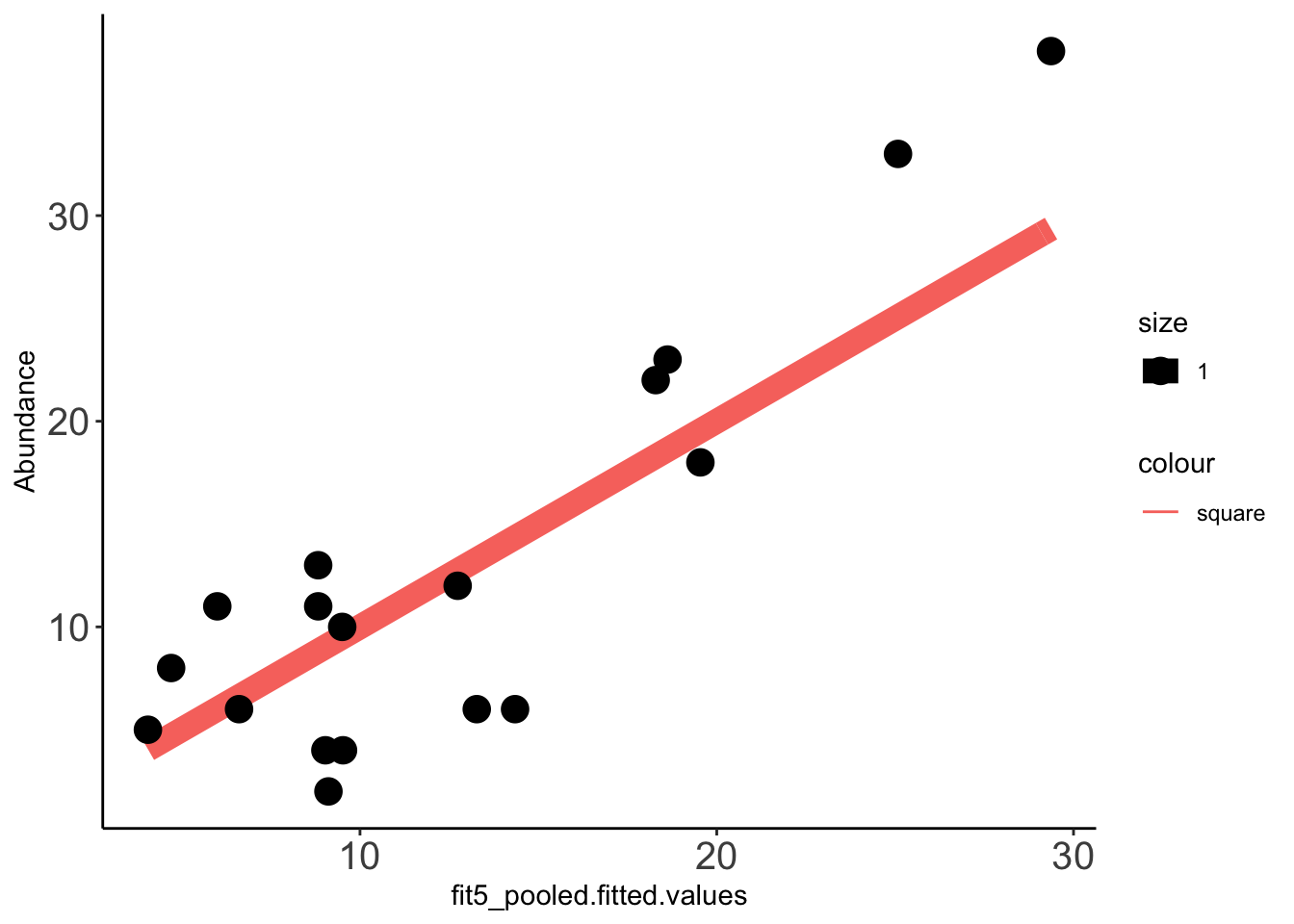
# ggplot(compicmut,aes(x=IC50,y=(drug_effect_obs^.5),label=Compound))+geom_text()

################Predictions using individual IC50s################
fit5<-glm.nb(Abundance ~ IC50+log10(Mutation.Probability), data=compicmut) #Best 2 variable model
summary(fit5)
Call:
glm.nb(formula = Abundance ~ IC50 + log10(Mutation.Probability),
    data = compicmut, init.theta = 8.493014642, link = log)

Deviance Residuals:
     Min        1Q    Median        3Q       Max
-1.88350  -0.86451   0.08648   0.42176   1.67167

Coefficients:
                             Estimate Std. Error z value Pr(>|z|)
(Intercept)                 5.247e+00  7.707e-01   6.809 9.84e-12 ***
IC50                        1.045e-04  4.022e-05   2.598  0.00939 **
log10(Mutation.Probability) 8.310e-01  2.040e-01   4.074 4.62e-05 ***
---
Signif. codes:  0 '***' 0.001 '**' 0.01 '*' 0.05 '.' 0.1 ' ' 1

(Dispersion parameter for Negative Binomial(8.493) family taken to be 1)

    Null deviance: 48.126  on 17  degrees of freedom
Residual deviance: 18.618  on 15  degrees of freedom
AIC: 116.2

Number of Fisher Scoring iterations: 1

              Theta:  8.49
          Std. Err.:  5.17

 2 x log-likelihood:  -108.201
Data_fit=data.frame(cbind(Data_fit,fit5$fitted.values))
x=ggplot(data =Data_fit,aes(fit5.fitted.values,Abundance))
x+stat_function(fun=function(x)x, geom="line", aes(colour="square",size=1.0))+geom_point(aes(size=1))+theme_classic()+theme(axis.text.x = element_text(size=15),axis.text.y = element_text(size=15))Warning: `mapping` is not used by stat_function()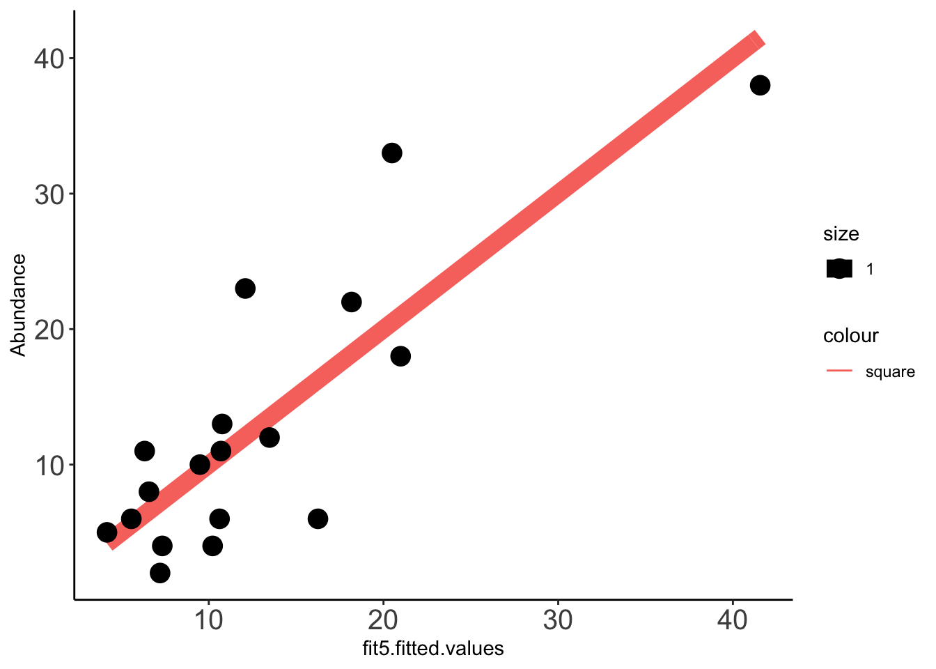
| Version | Author | Date |
|---|---|---|
| c2930d5 | haiderinam | 2020-04-03 |
#########Plotting predictions from inidivual IC50s and pooled experiments on the same plane#########
x=ggplot(data =Data_fit,aes(fit5.fitted.values,Abundance,label=Compound))
plotly=x+stat_function(fun=function(x)x, geom="line", aes(colour="square",size=1.0))+geom_text(aes(size=1,color="blue"))+geom_text((aes(x=fit5_pooled.fitted.values,size=1.0,color="green")))+theme_classic()+theme(axis.text.x = element_text(size=15),axis.text.y = element_text(size=15))
Warning: `mapping` is not used by stat_function()ggplotly(plotly)####Pearson's correlations
cor(Data_fit$fit5_pooled.fitted.values,Data_fit$Abundance,method="pearson")[1] 0.8805886cor(Data_fit$fit5.fitted.values,Data_fit$Abundance,method="pearson")[1] 0.8312331Predicting clinical abundances using the best spike-in mix
#Using just the experiment that ended up giving us the best growth rates.
mean_netgr=twinstrand_simple_melt_merge%>%filter(experiment%in%c("M3"),duration%in%("d3d6"))
mean_netgr=mean_netgr%>%filter(!netgr_obs%in%NA)%>%
  dplyr::select(mutant,netgr_obs)


compicmut2=merge(compicmut,mean_netgr,by.x ="Compound",by.y="mutant")
# compicmut2$IC50=compicmut2$netgr
compicmut=compicmut2
#Notice that value here is your fitted IC50s
################Predictions using pooled IC50s################
# fit5_pooled<-glm.nb(Abundance ~ netgr_mean+(Mutation.Probability), data=compicmut)
# summary(fit5_pooled)
fit5_pooled<-glm.nb(Abundance ~ netgr_mean+log10(Mutation.Probability), data=compicmut)
############Adding the CIs of predictions and plotting################
# Could have used confint(fit5_pooled)
linkinv=family(fit5_pooled)$linkinv #Using the inverse link function. Whatever the fuck that means. Got it from here https://stackoverflow.com/questions/35235939/how-to-plot-logistic-glm-predicted-values-and-confidence-interval-in-r
pred=predict(fit5_pooled,newdata=compicmut,type="link", se.fit = T)

upper=linkinv(pred$fit)+(1.96*pred$se.fit)
lower=linkinv(pred$fit)-(1.96*pred$se.fit)

Data_fit=data.frame(cbind(compicmut,fit5_pooled$fitted.values)) ###Need to check that doing a cbind this way makes the right mutants go to the right row in compicmut. Pretty sure it does.
Data_fit=cbind(Data_fit,upper,lower)

x=ggplot(data =Data_fit,aes(fit5_pooled.fitted.values,Abundance))
x+stat_function(fun=function(x)x, geom="line", aes(colour="square",size=1.0))+geom_point(aes(size=1))+theme_classic()+theme(axis.text.x = element_text(size=15),axis.text.y = element_text(size=15))
Warning: `mapping` is not used by stat_function()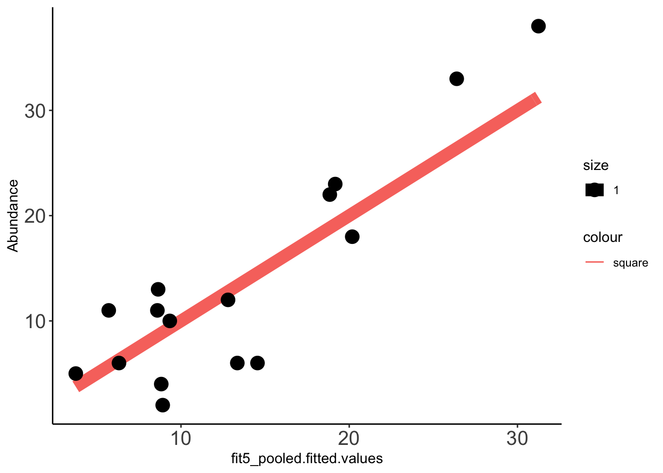
# ggplot(compicmut,aes(x=IC50,y=(drug_effect_obs^.5),label=Compound))+geom_text()
############Saving Predictions using pooled IC50s as a BMES figure################
x=ggplot(data =Data_fit,aes(Abundance,fit5_pooled.fitted.values))
x+geom_abline()+
  # stat_function(fun=function(x)x, geom="line", aes(colour="square",size=1.0))+
  # geom_point(aes(size=1))+
  geom_point(aes(alpha=.7))+
  geom_errorbar(aes(ymin=lower,ymax=upper))+
  scale_y_continuous(name="Model Predicted Clinical Abundance",limits=c(0,40))+
  scale_x_continuous(name="Clinical Abundance",limits=c(0,40))+
  theme_classic()+
  theme(axis.text.x = element_text(size=15),
        axis.text.y = element_text(size=15))+
  cleanup+
  theme(legend.position = "none")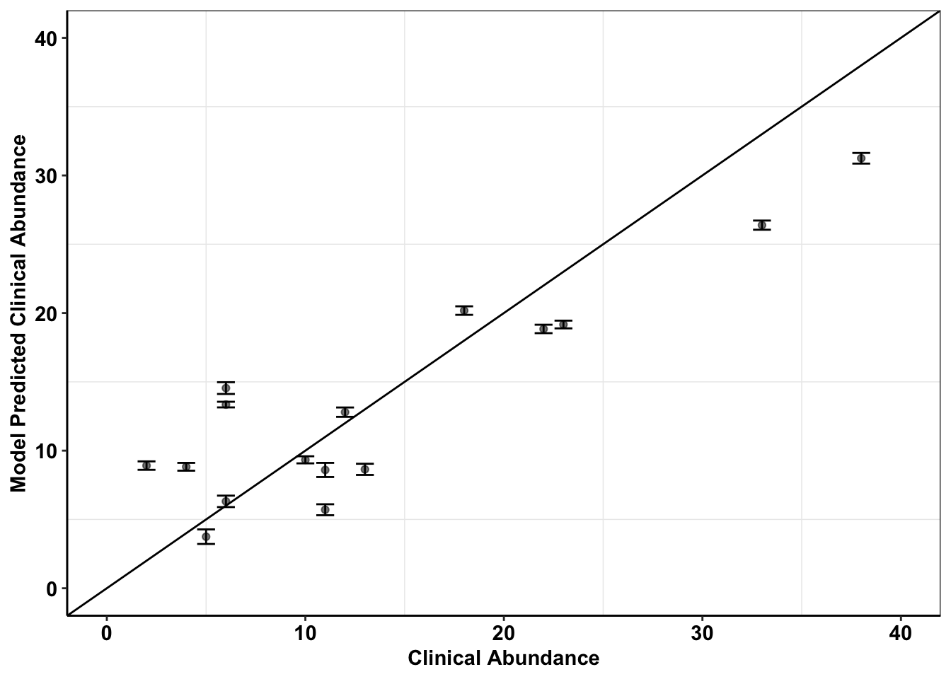
| Version | Author | Date |
|---|---|---|
| c2930d5 | haiderinam | 2020-04-03 |
# ggsave("clinicalabundancepredictions_BMES_abstract_51320.pdf",width=2,height=2,units="in",useDingbats=F)
################Predictions using individual IC50s################
fit5<-glm.nb(Abundance ~ IC50+log10(Mutation.Probability), data=compicmut) #Best 2 variable model
summary(fit5)
Call:
glm.nb(formula = Abundance ~ IC50 + log10(Mutation.Probability),
    data = compicmut, init.theta = 9.531288067, link = log)

Deviance Residuals:
     Min        1Q    Median        3Q       Max
-2.06327  -0.56673   0.08711   0.34958   1.59965

Coefficients:
                             Estimate Std. Error z value Pr(>|z|)
(Intercept)                 5.398e+00  7.590e-01   7.111 1.15e-12 ***
IC50                        9.498e-05  3.963e-05   2.397   0.0165 *
log10(Mutation.Probability) 8.578e-01  2.026e-01   4.235 2.29e-05 ***
---
Signif. codes:  0 '***' 0.001 '**' 0.01 '*' 0.05 '.' 0.1 ' ' 1

(Dispersion parameter for Negative Binomial(9.5313) family taken to be 1)

    Null deviance: 45.705  on 15  degrees of freedom
Residual deviance: 16.734  on 13  degrees of freedom
AIC: 105.04

Number of Fisher Scoring iterations: 1

              Theta:  9.53
          Std. Err.:  6.35

 2 x log-likelihood:  -97.039
Data_fit=data.frame(cbind(Data_fit,fit5$fitted.values))
x=ggplot(data =Data_fit,aes(fit5.fitted.values,Abundance))
x+stat_function(fun=function(x)x, geom="line", aes(colour="square",size=1.0))+geom_point(aes(size=1))+theme_classic()+theme(axis.text.x = element_text(size=15),axis.text.y = element_text(size=15))Warning: `mapping` is not used by stat_function()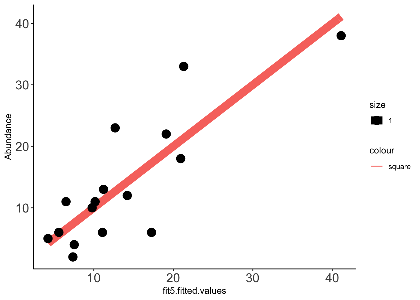
#########Plotting predictions from inidivual IC50s and pooled experiments on the same plane#########
x=ggplot(data =Data_fit,aes(fit5.fitted.values,Abundance,label=Compound))
plotly=x+stat_function(fun=function(x)x, geom="line", aes(colour="square",size=1.0))+geom_text(aes(size=1,color="blue"))+geom_text((aes(x=fit5_pooled.fitted.values,size=1.0,color="green")))+theme_classic()+theme(axis.text.x = element_text(size=15),axis.text.y = element_text(size=15))
Warning: `mapping` is not used by stat_function()ggplotly(plotly)####Pearson's correlations
cor(Data_fit$fit5_pooled.fitted.values,Data_fit$Abundance,method="pearson")[1] 0.8939072cor(Data_fit$fit5.fitted.values,Data_fit$Abundance,method="pearson")[1] 0.8379013Supplemental Analysis
enu_plots=twinstrand_simple_melt_merge%>%filter(experiment%in%c("Enu_4","Enu_3"),duration%in%"d3d6")
#hardcoding adjustments to the growth rates
enu_plots$netgr_obs[enu_plots$experiment=="Enu_3"]=enu_plots$netgr_obs[enu_plots$experiment=="Enu_3"]-.011

a=twinstrand_simple_melt_merge%>%
  filter(!experiment%in%c("Enu_4","Enu_3"),duration%in%"d3d6",conc=="0.8")%>%
  mutate(netgr_obs=case_when(experiment=="M5"~netgr_obs+.015,
                                   experiment%in%c("M3","M6","M5","M4","M7")~netgr_obs))

a_sum=a%>%group_by(mutant,Spike_in_freq)%>%summarize(mean_netgr_pred=mean(netgr_pred),mean_netgr_obs=mean(netgr_obs),sd_netgr_obs=sd(netgr_obs),mean_drug_effect=mean(drug_effect_obs),sd_drug_effect=sd(drug_effect_obs),mean_drug_effect_pred=mean(drug_effect),sd_drug_effect_pred=sd(drug_effect))

plotly=ggplot(a_sum,aes(x=mean_netgr_pred,y=mean_netgr_obs,color=factor(Spike_in_freq)))+geom_errorbar(aes(ymin=mean_netgr_obs-sd_netgr_obs,ymax=mean_netgr_obs+sd_netgr_obs))+geom_point()+geom_point(data=enu_plots%>%filter(experiment%in%("Enu_3")),aes(x=netgr_pred,y=netgr_obs,color="red"))+geom_abline()+cleanup
ggplotly(plotly)
####Plotting drug effect on growth rate rather than net growth rate
plotly=ggplot(a_sum,aes(x=mean_drug_effect_pred,y=mean_drug_effect,color=factor(Spike_in_freq)))+geom_errorbar(aes(ymin=mean_drug_effect-sd_drug_effect,ymax=mean_drug_effect+sd_drug_effect))+geom_point()+geom_abline()+cleanup
ggplotly(plotly)plotly=ggplot(a_sum%>%filter(!Spike_in_freq%in%c(5000)),aes(x=mean_drug_effect_pred,y=mean_drug_effect,color=factor(Spike_in_freq)))+geom_errorbar(aes(ymin=mean_drug_effect-sd_drug_effect,ymax=mean_drug_effect+sd_drug_effect))+geom_point()+geom_abline()+cleanup
ggplotly(plotly)plotly=ggplot(a_sum,aes(x=mean_drug_effect_pred,y=mean_drug_effect,color=factor(mutant)))+geom_errorbar(aes(ymin=mean_drug_effect-sd_drug_effect,ymax=mean_drug_effect+sd_drug_effect))+geom_point()+geom_abline()+cleanup
ggplotly(plotly)
sessionInfo()R version 4.0.0 (2020-04-24)
Platform: x86_64-apple-darwin17.0 (64-bit)
Running under: macOS Catalina 10.15.4
Matrix products: default
BLAS: /Library/Frameworks/R.framework/Versions/4.0/Resources/lib/libRblas.dylib
LAPACK: /Library/Frameworks/R.framework/Versions/4.0/Resources/lib/libRlapack.dylib
locale:
[1] en_US.UTF-8/en_US.UTF-8/en_US.UTF-8/C/en_US.UTF-8/en_US.UTF-8
attached base packages:
[1] stats graphics grDevices utils datasets methods base
other attached packages:
[1] plotly_4.9.2.1 dplyr_0.8.5 boot_1.3-24
[4] lme4_1.1-23 Matrix_1.2-18 fitdistrplus_1.0-14
[7] npsurv_0.4-0.1 lsei_1.2-0.1 survival_3.1-12
[10] MASS_7.3-51.5 ggplot2_3.3.0 lmtest_0.9-37
[13] zoo_1.8-8
loaded via a namespace (and not attached):
[1] statmod_1.4.34 tidyselect_1.1.0 xfun_0.13 purrr_0.3.4
[5] splines_4.0.0 lattice_0.20-41 colorspace_1.4-1 vctrs_0.3.0
[9] viridisLite_0.3.0 htmltools_0.4.0 yaml_2.2.1 rlang_0.4.6
[13] later_1.0.0 pillar_1.4.4 nloptr_1.2.2.1 glue_1.4.1
[17] withr_2.2.0 lifecycle_0.2.0 stringr_1.4.0 munsell_0.5.0
[21] gtable_0.3.0 workflowr_1.6.2 htmlwidgets_1.5.1 evaluate_0.14
[25] labeling_0.3 knitr_1.28 crosstalk_1.1.0.1 httpuv_1.5.2
[29] Rcpp_1.0.4.6 promises_1.1.0 scales_1.1.1 backports_1.1.7
[33] jsonlite_1.6.1 farver_2.0.3 fs_1.4.1 digest_0.6.25
[37] stringi_1.4.6 grid_4.0.0 rprojroot_1.3-2 tools_4.0.0
[41] magrittr_1.5 lazyeval_0.2.2 tibble_3.0.1 tidyr_1.0.3
[45] crayon_1.3.4 whisker_0.4 pkgconfig_2.0.3 ellipsis_0.3.1
[49] data.table_1.12.8 httr_1.4.1 assertthat_0.2.1 minqa_1.2.4
[53] rmarkdown_2.1 R6_2.4.1 nlme_3.1-147 git2r_0.27.1
[57] compiler_4.0.0